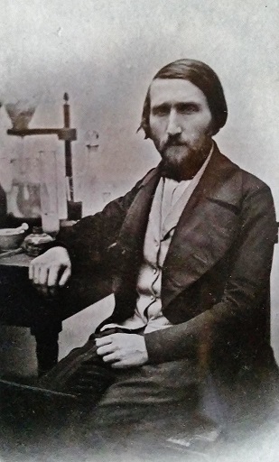
The Italian chemist Francesco Selmi in his laboratory, a XIX century scientific worker
Today May 1st, the international workers’ day, is the perfect day to reflect on the role of the worker, that is, of the one who lives from his or her work, operating on the environment and on society, more and more often through a computer. My thesis is that to survive and thrive in the current and future world, under the impacts of climate change, and the technological disruptions brought by artificial intelligence and quantum computers, the worker must transform herself into a scientific worker. The main activity of this new kind of worker is to learn, in order to act in a conscious, rational and effective manner, in harmony with the society and the environment. In the followings, after a short premise, I have reported a list of topics that I consider fundamental to master for the scientific worker (naturally among these there is also English). I have put the adjective “scientific” in parentheses in the title because every worker will have to be a scientist, and continuously learn, so that there should be no need to use the adjective.
The new worker
The modern worker must be able to read and interpret the data coming from the environment: physical, social, economical and financial environment. The data must be available in digital format, open and easily usable by computing machines. The worker must be able to read, transform, interpret, and produce data. In order to possess these skills the worker must have a good and actionable knowledge of mathematics, physics, biology, finance, and computer science. Here follows a list of topics that, according to my experience, a scientific worker should grasp.
Mathematics
Propositional and predicate calculus
Real and complex analysis
Calculus
Linear Algebra
Geometry
Probability distributions
Differential equations
Graph theory
Optimization and linear programming
Data assimilation, transforms, inversion and interpolation
This knowledge is fundamental, independently of the economy in which the (scientific) worker operates, that is, market or socialist economy.
Education and culture
Open and machine readable data is not enough. The cost of education should be kept at its minimum and I appreciate those who publish their scientific work freely online. I publish a collection of high quality textbooks made freely available by their authors here on my website. One more important characteristic of the (scientific) worker is a knowledge sharing culture. For this reason I have organized the PyData Rome group on Meetup.
Conclusion
If you see yourself as a (scientific) worker you are invited to join the PyData Rome group today. Happy international workers’ day!
]]>The PyData Rome Chapter: Ideas and Commitments2023-01-27T00:00:00+00:002023-01-27T00:00:00+00:00/pydata/pydata-rome-chapter
What is PyData ?
PyData is an educational program of NumFocus, a nonprofit charity promoting open practices in research, data, and scientific computing. It provides a forum for the international community of users and developers of data analysis tools to share ideas and learn from each other. The forum is organized on the Meetup platform and currently, in January 2023, there are 215 groups in 73 countries.
The Rome PyData Chapter
The Rome PyData chapter started in September 2022 and had its first meeting in December 2022 thanks to the support of Binario F, an innovation laboratory managed by Facebook in the center of Rome that provided us with the facility for our meeting. The PyData Rome chapter was started out of a lack of events related to computational science, open source software development, and open data in our city. Our aim is to contribute to change the landscape of the city for what is related to open science and awareness of new technologies and the opportunities they bring.
Changing the landscape
There are many Italian newspaper articles and blog posts that talk about machine learning and artificial intelligence but not many opportunities to learn to become an active user and not just a passive or even unaware consumer of such technologies. We want to fill that gap. Rome has almost 4 million inhabitants, three universities with a total of more than 100k students, and many research institutions. Furthermore, many large private, public and international organizations, that deal with increasing amounts of complex data, have their headquarters here. We need more people able to work on these data sets and more opportunities to learn and share ideas. If we look at other PyData chapters in Europe we see a correlation between the numbers of their members and events that they organize and the country’s leadership in innovation, open science, and technology.
Ambitions
The PyData chapters in London, Berlin, Amsterdam, and Paris are leading the ranking in Europe by their number of members (4k to 11k) and events they have organized in 2022 but others such as Copenhagen and Madrid are performing well too. We think Rome has everything it needs to be in this group and we have committed ourselves to have at least one meeting per month to help our city to move up.
PyData Meetup
Members
Events (2022)
Attendees
London
11756
5
832
Berlin
7139
8
817
Amsterdam
4659
6
496
Paris
4109
7
297
Copenhagen
2165
9
499
Madrid
1092
9
278
Rome
52
1
12
Open to contributions
If someone in Rome shares our same ideas and is willing to support our efforts by hosting our meetings or contributing to an event with a proposal, let’s get in contact on our page on Meetup or meet directly in one of our next events!
So we managed to have our 1st PyData Rome meeting. We started the Rome chapter of the PyData community in September. The group on Meetup counts 31 members right now. There were 12 members that subscribed to participate and 3 of them eventually found their way to the meeting room hosted at Binario F, an initiative by Facebook to provide a physical space for business and individual development in Rome. You may say that was a failure, as only three people came to the meeting. No, I say it was a success: 25% of those who subscribed came, and two others wrote to me thinking it was online (sorry guys!).
Numbers are not the most important metric for a meeting
First of all, I had fun in preparing the presentation and meeting with other like-minded people. We had an interesting talk before the beginning of the presentation, during its delivery and after it. Beyond the technical discussion about Deep Learning and satellite imagery we had a very interesting conversation about the lack of opportunities for developers interested in data science to meet and share ideas outside of an academic environment in Rome. That is exactly what we want to address with the PyData Rome chapter. Rome is not San Francisco but there are three universities with data science departments full of smart people and one of this, the Sapienza University of Rome is one of the largest European universities. So it’s not the lack of people, it’s the culture, the idea hidden in our mind that participating in these events after you leave your academic institution and start to work doesn’t really matter anymore.
Participation matters
We are here to say it does matter. It matters because we have to be lifelong learners if we want to make contributions to society and keep control of our working life. One other important aspect is that science is too much a relevant enterprise to be left exclusively to academic institutions. There must be a collaboration between academic institutions and people, citizens, and private organizations that are interested in science, not a wall or a border that cannot be crossed. There are several critical problems to be addressed for which our societies need people able to invent and apply algorithms to make sense of the data coming from satellites and other sensors. This is the mission of the PyData community and the reason for which we joined.
Learning is fun
Last but not least, learning is fun and using what we learn for things that matter with other people is even more fun. In conclusion, I want to thank the participants, Binario F, the people who helped to set up the room for the presentation, and in particular Matteo Franza who manages the space and provided us an excellent room for our meeting.
(The slides used for the presentation with links to code and other materials are available here)
The Roman Forum close to the Capitolium, venue of the 3rd day of the Conference
The 10th annual SISC conference on climate change, SISC2022: Governing the Future is over. Friday 21st was the 3rd and last day of the conference held at the Protomoteca hall at the Rome’s Capitolium. This is the 1st year I participate in the conference with a work about land use and classification using satellite optical images and a convolutional neural network. Climate change is not only a scientific topic. As everyone is experiencing or witnessing its consequences on the environment, a lot of studies and research are dedicated on how to address its impacts on health, food production, the economy and society in general at different scale, from a global perspective to a local one and in particular on urban areas. This is the first time the conference was held offline since 2019. In three days I had the opportunity to learn about the research work that is being pursued in areas in which I have little or no knowledge at all, such as food production in ocean waters and policies studies for adaption and mitigation actions. I had also the opportunity to meet many people that work on different issues related to climate change. I’d like to mention Riccardo Valentini, professor of Forest Ecology at the Tuscia University, a leading author of the 5th IPCC report and winner of the 2007 Nobel Prize for Peace as a member of the IPCC board; Antonello Pasini, climate change scientist at the Institute of Atmospheric Pollution Research of the National Research Council, author of several books on climate change and its impacts on our planet, blogger at the Le Scienze and speaker in many broadcasting services; Mita Lapi, coordinator of the Sustainable Development Department at the Lombardy Foundation for the Environment. Mita took part on a field work on the Adamello glacier that was presented at the conference and told me how the Italian Society for Climate Sciences was born as a place for researchers and institutions working on the many different facets of climate change to meet, share their knowledge and collaborate. A side event that was held at the Capitolium was about Cities and Climate and had as invited speakers Francesco Rutelli, former mayor of Rome, journalists and current administrators of the city. Rutelli made many sensible statements, one particularly relevant and not always mentioned was that if we want to move away from a fossil fuels based economy, governments and industries have to foster the kind of productions that are inevitably going to replace the old ones and take into account the social impacts of such changes for example by re-training the people that will loose their jobs in the old economy in order to be able to work in the new one. There is a strong need to adapt cities like Rome to the climate change and one is to replace fossil fuels with renewable sources such as solar panels. Rome has 245 $Km^2$ of built areas, 19% of its territory, of which 45.5 $Km^2$ are buildings so I asked one of the city’s administrators if there is any study to assess the feasibility of installing solar panels on the roofs of such buildings. He told me there is not yet such study. I think this is one of the many tasks in which satellite images and machine learning algorithms can help citizens and decision makers to make the best decisions on our path to a new world. This might be my inspiration for some future work on Deep Learning.
In conclusion, this was my first conference in the city in which I was born and it was a great experience. I do believe that Rome is a very good place to work on climate change issues, not only because international organizations such as The UN-FAO, the World Food Programme, and ESA-ESRIN have here their headquarters, but also because Rome can be a laboratory for governing the future instead of being passively brought to adverse and unpleasant scenarios.
]]>Spatial Relations in GeoPandas2022-10-04T00:00:00+00:002022-10-04T00:00:00+00:00/geoscience/spatial-relationsHumans have the ability to figure out the spatial relations of objects in their visual field without any effort. It is certainly an evolutionary characteristic that has been embedded in our brain because of its importance in many common reasoning tasks. Since objects can be represented in computer systems, algorithms have been developed over the years to support the same functions.
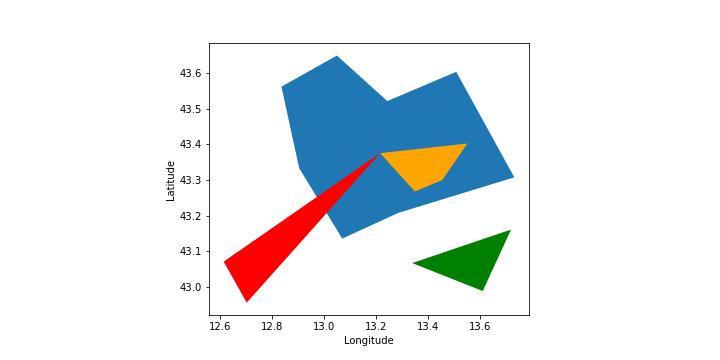
In many applications of geoscience, for example in emergency management or risk assessment, one wants to know the spatial context of the area in which a certain event occurred and link the spatial information to external data sources through a named entity. For example, it is not enough to know the extent of a flooded area, we want to know in which administrative region it lies, or we might want to know the distance of a wildfire from a real estate or a populated area. In other words, we want to know the spatial relation between the area in which an event occurred and the area that belongs to or is run by a owner or authority. This post describes the notebook that I have developed on the implementation of spatial relations in GeoPandas. The reader can go directly to the Jupyter notebook in case she or he wants to see the code. We will deal only with topological relations, a subclass of spatial relations that don’t need a metric, that is a way to compute the distance between two spatial objects. The notebook starts by creating some simple spatial objects, points and polygons, to see what kind of topological relations can be established between them. Finally, the topological relations will be tested between our abstract layers, blue, red, orange and green, and the geometry of Marche, one of the 20 regions of Italy, and of its administrative units, i.e. the municipalities.
Python packages
Spatial objects such as points, lines and polygons, may have one or more topological relationships such as contains, overlap, within, touches. The Python package Shapely, included in GeoPandas, implements such functions for points, lines and polygons. Shapely is a Python port of GEOS, the C++ port of the Java Topology Suite (JTS), a Java implementation of topological relations. We start by importing the Python packages we are going to use. We use the minimum set of packages to get the job done.
Coordinate reference systems
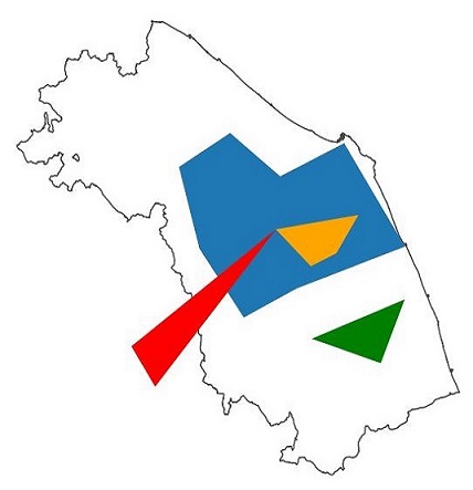
Even if establishing the topological relationship between two spatial objects doesn’t involve a metric, objects must be represented using the same coordinate reference system (CRS). We will create some spatial objects using the unprojected reference system WGS84 EPSG:4326. We will also import two datasets: the border of the Marche region and the borders of its administrative units, the municipalities of the region. We will see what spatial relations exists between our abstract layers and the Marche region and its administrative units. The two datasets have their own CRS whose ESPG code is EPSG:32632. This CRS is projected on a 2D surface using the Transverse Mercator projection and the unit of measure is the meter so, in order to use the spatial relationships between the spatial objects of our layers and the polygons of the Marche region and its administrative units we will have to change the CRS of our layers to be the same as that used for the region and its municipalities and transform the coordinates of points and polygons accordingly.
Spatial joins
Spatial relations are used to merge two spatial datasets A and B in which each row of A and B contains spatial objects. The merge can be based on one topological relation such as “contains”, so that if object i of A contains object i of B, the value in one or more columns of B will be added to the object in A. We will not deal with spatial joins here since it’s an application of the topological relations.
Spatial objects, areas of interest, and layers
We will use spatial objects such as Points, Lines and Polygons for which a set of coordinate pairs will be assigned. A layer is a collection of one or more spatial objects that describes a certain event that occurred over an area of interest. In GeoPandas a layer is built using a GeoDataFrame. A GeoDataFrame is a subclass of the DataFrame class of the Pandas Python library that has a column with geometry.
Topological relations
We apply the topological relations: within, intersects and touch between the polygons that we have defined. We will not use contains since it’s the inverse of within. We will apply the topological relations to pairs of polygons from two different layers. The methods take the left operand from a polygon of one layer and the right operand from the corresponding polygon of the other layer. By “corresponding” we mean the polygons have the same index value in the two GeoDataFrame used to implement our layers.
within
From the relation definition in Geopandas: “An object is said to be within another if at least one of its points is located in the interior and no points are located in the exterior of the other.”
intersects
From the relation definition in GeoPandas: “An object is said to intersect another if its boundary and interior intersects in any way with those of the other.”
touches
From the relation definition: “An object is said to touch another if it has at least one point in common with other and its interior does not intersect with any part of the other. Overlapping features therefore do not touch.”
Projections
When we want to apply the topological relations to spatial objects from different layers (GeoDataFrame) we have to check that the coordinate reference system (CRS) used in the two layers is the same. In the following sections we will use two datasets that use the Transverse Mercator projection (EPSG:32632). Since our colored layers use the WGS84 unprojected CRS (EPSG:4362) we will have to change it and use the EPSG:32632. When we change the CRS GeoPandas transforms the coordinates of the points automatically. The coordinate units in the Transverse Mercator projection is in meters instead of degrees.
Spatial relations in the real world
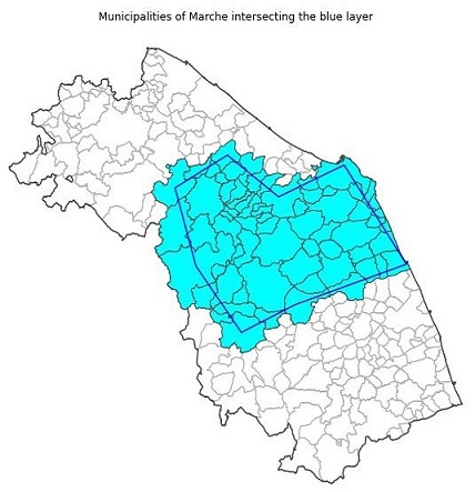
Our points and polygons in the blue, red, orange and green layers are not completely abstract. They represent towns and areas in the Marche region. We want to find out which spatial relationships between them, the Marche region and its administrative units, the municipalities, hold true and which do not.
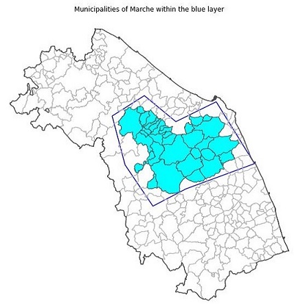
Municipalities of the Marche region
We want to see which municipality lies within the polygon of the blue layer. We start by opening the dataset of the municipalities of the Marche region. This dataset has been extracted from the dataset of the Italian municipalities from ISTAT, the Italian National Institute of Statistics and it is available in the data folder of the repository.
Municipalities of Marche within the blue layer
Municipalities of Marche intersecting the blue layer
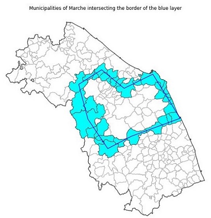
Further logic operations with masks
As we can see the within relationship is stronger than intersects. We might want to see only the municipalities that intercept the blue area but are not completely within it. With GeoPandas such logic operation can be done with one line of code.
border_intersects = intersects & ~within
Conclusion
We have seen some examples of spatial relations between polygons in GeoPandas. We have applied such relations to geometries of the municipalities of the Marche region in Italy. We have changed the coordinate reference system of our example layers to be the same as that used for the Marche region and its administrative units. We have also performed a further logical operation dividing the geometries of the municipalities that strictly intersect one of our fictional layer from those that lie completely in our layer using logical operators on the result of the spatial relations. Spatial relations are fundamental to perform spatial analysis over multiple layers. We want to underline that they also provide a mean to integrate the information about events, such as flooded areas, with contextual information from external data sources by using the name or identifier of a named entity whose geometry has a spatial relation with the event. As said in the introduction the Jupyter notebook with the Python code used for this post is available on my GitHub repository.
This post contains my notes from the webinar “Recent Development in S6 Altimetry Measurement” organized by EUMETSAT the 29th September 2022 with Ben Loveday, Vinca Rosmorduc, Christine Traeger Chatterjee and Hayley Evers-King. The webinar took place on Zoom. Q&A on Slido (code #EUMSC33). The training provided by EUMETSAT is fundamental to those who want to use the data that is made available by the ESA under an open data policy.
Sentinel-6 Radar Altimetry
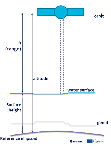
Sentinel-6 is a satellite dedicated to the measurement of the sea level and significant wave height. The first satellite was launched in November 2020, a second satellite is expected to be launched in 2025. The Sentinel-6 altimeter is an improved version of the SRAL altimeter on board the Sentinel-3 satellites. The technique used for the observations is radar altimetry. The technique can also be used to monitor the level of natural and artificial water bodies (i.e. lakes and dams), snow and ice sheets. The webinar focused on the marine domain. The main payload of Sentinel-6 is a Poseidon-4 synthetic aperture radar looking at nadir that works on two bands: Ku band (13.575 GHz, or 2.2 cm wavelength) and C band (5.41 GHz, or 5.5 cm wavelength). A very simplified idea of the technique can be gained from what follows. The radar on board of the satellite sends electromagnetic pulses that after a certain amount of time reach the sea surface from which are reflected backwards, and after an equal amount of time hit the radar antenna. The distance, or range, of the satellite from the sea surface can be computed knowing the speed of light
\[range = \frac{c * \tau }{2}\]
where $\tau$ is the travel time of the pulse from the radar to the sea surface and back, and $c$ is the speed of light. Once we have the range between the satellite and the sea surface, we can compute the height of the sea surface from the reference ellipsoid, the mathematical model that represents the shape of the Earth, from the difference between the altitude of the satellite, that is its distance from the same reference ellipsoid, and the range
The satellite also hosts a GNSS system for precise orbit and altitude determination, and a microwave radiometer used to determine the error on the measure of the path of the radar signal due to the water vapor in troposphere. The (goal) resolution in height measurement is 0.5 cm, the resolution achieved so far is 0.62 cm. The along-track resolution is 50 cm. The along-track resolution is relevant for coastal sea level measurements, less relevant in the open sea. The sea level rise that has been observed so far is 3.53 mm/year, that is more than 1 cm every three years, an alarming value that tells us a lot about the relevancy of these observations.
Data Products and Service with Python Client and Examples
The Sentinel-6 products are released through the EUMETSAT Data Service. By searching for “Altimetry” on the user interface the Sentinel-6 products can be found and downloaded. A web service is also available for programmatic access to the data. Examples on how to access the service using the EUMDAC Python client are given on the EUMETlab platform with examples on how to use the Sentinel-6 products. The documentation is available on EUMETSAT JIRA platform
Q&A Session
Questions have been written on slido.com and the answers are available in the video recording of the webinar.
Resources
A good resource to learn about radar altimetry, in addition to the slides by Vinca Rosmorduc presented in the webinar, is the book by Iain H. Woodhouse, Introduction to Microwave Remote Sensing, that dedicates 16 pages to radar altimeters. Other resources are available on the altimetry.info website with a tutorial about the applications of radar altimetry.
Notebooks, where working code is mixed with text and visualizations, are powerful tools to test and share ideas with a quantitative approach in mind. Wekeo is one of the European Data and Information Access Service (DIAS) that provides computing resources and easy access to the Copernicus data, services and satellite imagery. It is extremely important for Europe to provide such services and be competitive with US companies in exploiting the value of the Copernicus data released under an open data policy. In my notebooks I use three datasets from the Copernicus services to extract three essential climate variables: the near surface air temperature, the solar radiation and the nitrogen dioxide. The air temperature is a key indicator of climate change, is the heat we feel and that, as we all know, is increasing because of the global warming. The solar radiation is the energy that hits the Earth surface after it goes through the atmosphere and the clouds. It is useful to decide what should be the size of a solar power plant to produce enough energy or hot water to support the consumption of a family or community in a sustainable way. Finally, the nitrogen dioxide is an indicator of the air pollution. I hope my notebooks will be helpful to those who are interested in using the Copernicus data.
19th Oct. 2022 Solar Radiation Notebook Awarded the 3rd Prize of the Wekeo JNC
I am glad to say that one of my notebooks, the one on solar radiation, won the 3rd place of the Wekeo Jupyter Notebook competition. Thanks to Dr. Hayley Evers-King, Christopher Stewart and the team from Copernicus, EUMETSAT, ECMWF, Mercator Ocean for the nice award ceremony (video from 8:05) and certificate.
]]>ECRS 2022 Best Presentation Award2022-07-27T00:00:00+00:002022-07-27T00:00:00+00:00/copernicus/ecrs2022-best-presentation-award
The content of my presentation: I provide some tips for people interested in using Synthetic Aperture Radar imagery to estimate the extent of flooded areas. You do not have to be an expert on electromagnetic theory or digital image processing.
The delivery: my tips on how to prepare and deliver a successful presentation.
The content
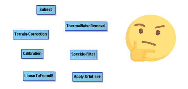
I have been working on Synthetic Aperture Radar (SAR) imagery from the Copernicus Sentinel-1 satellite for some time and I have found that the gap between the theory that can be learnt from textbooks and the practical knowledge needed to use the data in its many applications is very large. The people interested in using the free SAR data provided by the European Space Agency (ESA) through its Copernicus programme are not anymore only electronic engineers or physicists with a solid understanding of electromagnetic theory. Synthetic Aperture Radar is a very powerful technology that allows the monitoring of many natural and human-made phenomena such as floods, oil spills, subsidence, urbanization, volcanic eruptions, landslides, deforestation, glaciers and sea ice sheets melting. Given its broad range of applications SAR data users have a large variety of backgrounds: GIS analysts, natural resource managers, geologists, environmental researchers, geographers, community managers, land use planners, farmers, economists just to mention a few categories. The SAR data products that can be downloaded from the Copernicus Open Access Hub have to undergo a quite complex digital image processing chain depending on the application.
In some applications such as for volcanic eruptions, landslides and subsidence the user needs the phase and the amplitude of the backscattered signal in order to detect a change that might have occurred over the Earth surface. The technique, called SAR interferometry, consists of counting the number of wavelengths of the radar backscatter signal along the path from the target to the antenna on board the satellite, before and after the event that caused the change. The difference in the number of wavelengths is a measure of the change occurred at the target area. In other applications such as for agriculture, forest mapping, urban areas monitoring and oil spills detection the user might need to estimate the change of the polarization of the backscattered radar signal. As I was working with the ESA Science Toolbox Exploitation Platform to process the Sentinel-1 imagery in the middle of July 2021, Germany was hit by a devastating flood that killed 184 people and caused damages estimated to be €40 billions. I was living in Bonn at that time, very close to the affected areas so I decided to use the imagery and the toolbox to assess the extent of flooded area. The tutorials available on the tool’s website were mostly addressed to people already skilled in remote sensing and digital image processing with detailed descriptions about the mathematical operators required to extract the flooded areas from the rest of the image but without a clear explanation of why those operators were required and in which order. I wrote some notes for myself putting together the sequence of operators required for the task at hand, among those available in the toolbox, with a short explanation of their function. After a couple of weeks I thought the notes might be useful to other people as well, not expert in SAR digital image processing, and I sent them to the STEP Forum. The notes were quite well received and added to the list of the Sentinel-1 Toolbox tutorials. I shared the link to the tutorial on a LinkedIn group interested in Earth Observation that was well appreciated and I decided to participate in the 4th International Electronic Conference on Remote Sensing with my tutorial. The content was ready but what about presenting it ?
The delivery
I have given many presentations in my work but I never had the feeling to be good at that. Finally I came to the conclusion that presenting is something to be learnt, not something we are naturally gifted. So I looked for some textbooks and online courses and finally I found the course I was looking for, that could help me to improve my slides and my speech: the Matt Garrity’s course Dynamic Public Speaking, freely available on the Coursera platform. It’s made up of four courses, not just one: an introductory part on rhetoric and the origin of public speaking, a course on how to organize and structure your presentation and slides, one about persuasive argumentation , and one last course on how to make an inspirational speech. In a few sentences what I learnt from the course:
Make it clear what is the message you want to deliver to your public.
Structure your speech. Provide an introduction, state the problem you are going to talk about and say what you have done to solve it. Provide a conclusion.
Do not add too much text to your slides, better no words at all than too many. Remember the adage “a picture is worth one thousand words”.
Do not read, never. Prepare the delivery of your presentation with someone else kind enough to listen to you or in front of a mirror.
Conclusion
SAR is a powerful technology with many applications and an increasing number of users with different backgrounds eager to use the data and the tools made available by the Copernicus programme. Each application exploits different properties of the electromagnetic radiation and of its interaction with the Earth’s surface that might be difficult to grasp without a long training on electromagnetic theory and digital image processing. The learning curve can be made much less steep by developing tutorials that contain the practical information on how to use a tool with the contextual information about the theory relevant to the specific application.
My slides for the presentation are available here. You can look for my tutorial on the ESA STEP website, section Sentinel-1 Toolbox (SAR Applications): Flood mapping using the Sentinel-1 imagery and the ESA SNAP S1-Toolbox, October 2021, or download it directly from my website A new version of the tutorial will be available soon.
]]>Deep Learning for Land Use and Land Cover Classification2021-09-01T00:00:00+00:002021-09-01T00:00:00+00:00/eo/land-use-land-cover-classification
MathJax.Hub.Config({
tex2jax: {
inlineMath: [['$','$'], ['\\(','\\)']],
processEscapes: true
}
});
My goal with this experiment was to test the accuracy of Convolutional Neural Networks to learn the spatial and spectral characteristics of image patches of the Earth surface extracted from satellite images for Land Use and Land Cover (LULC) classification tasks. To achieve my goal I used a transfer learning technique that consists of using a pretrained ResNet CNN architecture [1] and finetune it with the EuroSAT dataset [2], a collection of labelled satellite patch images extracted from the Copernicus Sentinel-2 satellites products. I used the Fastai deep learning library to write the Python code to train and validate the system, and Google Colab to execute it on a GPU. I have also performed some additional LULC classification tests using new images extracted from the Copernicus Sentinel-2 dataset products through the Sentinel-Hub EO-Browser. In the next four sections I provide some information about the LULC classification task, the Sentinel-2 satellites and their products, the EuroSAT dataset, and the finetuning technique. In the coding sections that follow I describe all the steps required to set up a deep learning architecture to accomplish the LULC task and to assess the accuracy of the results.
Land Use and Land Cover (LULC) classification
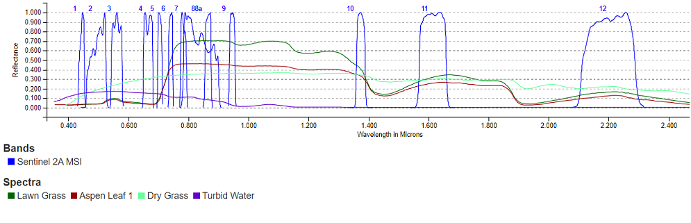
Land cover indicates the type of surface, such as forest or river, whereas land use indicates how people are using the land. Land cover can be determined by the reflectance properties of the surface. This information is commonly extracted from aerial or satellite digital images whose pixels values represent the solar energy reflected by the Earth’s surface in different spectral bands. The class of a land cover at the pixel level can be determined by using some combinations of spectral bands. For instance, vegetation has a stronger reflectance in the near infrared region of the spectrum and can be better observed using bands B7, B8, B8a and B9 of the Sentinel-2 MSI than the bands in the visible region of the spectrum, B4, B3, B2 (or RGB).
In the visible region, dry grass has a stronger reflectance in band 4 (Red) than in the other two bands B2 and B3 (blue and green). Classical machine learning algorithms such as Random Forests or Support Vector Machine are used to improve the accuracy of the classification. On the other hand, spectral data at the pixel level alone cannot provide information about the land use and a patch image has to be considered in its entirety to infer its use. Often also additional information is required to disambiguate among all the possible uses of a land. Different classification systems have been developed over the years whose goal is to define a taxonomy of land covers and land use. One such classification system is the CORINE land cover nomenclature [3] that contains 44 classes. CORINE is a land cover inventory performed every 6 years by the Copernicus Land Monitoring Service to monitor the changes in land use and land cover over the European continent. The maps produced by CORINE are based on the Sentinel-2 images classified at the pixel level according to the nomenclature and on information available from national cadastre. Since the availability of deep learning algorithms for computer vision, researchers have been developing models to perform LULC tasks, to be used at any time that new images are available and without using information from cadastre that might be expensive, not always up to date or not publicly available.
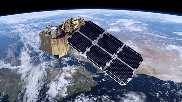
The Copernicus Sentinel-2 satellites
The Copernicus Sentinel-2 constellation is based on two identical satellites for earth observation, launched and operated by the European Space Agency (ESA). Each satellite flies on a Sun synchronous near-polar orbit at 786 km altitude, 180° apart from each other so that the same area can be revisited every 5 days. Both satellites carry a high spatial resolution multispectral imager (MSI) with a 290 km swath that can collect the solar energy reflected by the Earth surface in 13 spectral bands, from the visible to the near-infrared spectral range. The spatial resolution ranges from 10 m per pixel (B2, B3, B4, and B8 bands) down to 60 m per pixel. The ESA processes the raw data for radiometric calibration, orthorectification, atmospheric correction and georeferencing, and delivers the processed images as Level-1C (L1C) and Level-2A (L2A) data products. Both products are delivered as 100 km x 100 km tiles in UTM/WGS84 projection. L1C products are not processed for atmospheric correction and are described as Top-Of-Atmosphere reflectance data, while L2A products have received atmospheric correction and are described as Bottom-Of-Atmosphere reflectance data. L1C and L2A products can be obtained under an open access license from the Copernicus Open Access Hub or from other providers such as Sentinel-Hub.
Deep Learning Models
This section is meant to provide a very rough idea of the calculations used in Deep Learning to map an input to its output without any mathematical rigor. With this caveat in mind, it is known that a multilayer feedforward network, like ResNet50, can be used to build a model $y(x)$ to fit an unknown target function $y^*(x)$ that maps an input x to an output y. An input can be an image and the output a numeric value in case of a regression task or a categorical value in case of a classification task. The feedforward neural network model can be represented as nested functions, one function for each layer where the output of one layer’s units is the input to the following layer’s units. Each successive layer should provide a different and increasingly abstract view of the input. Let’s suppose we use a network with only three hidden layers where an input x goes from layer h to layer g and f
\[x → h → g → f → y(x)\]
Throwing mathematical precision to the winds, we can represent the model with the function
\[y(x, w) = f(g(h(x, w_h), w_g), w_f)\]
where w represents all the parameters $w_h, w_g, w_f$. We train our model using a data set of N inputs with labels {$x^{(n)}, t^{(n)}$} that represent a sample of the unknown function $y^*(x)$. Our model should minimize a cost function
\[ℒ = \frac{1}{2}||y(x, w) - y^*(x)||^2\]
One algorithm used to minimize the cost function is gradient descent with backward propagation
\[w_{i+1} = w_i - γ∇_wℒ\]
where i is the index of a batch of inputs used to update the parameters w, $γ$ the learning rate, and
\[∇_wℒ = ||y(x, w) - y^*(x)|| ∇_wy\]
The gradient $∇_wy$ is computed following the chain rule from Calculus implemented in PyTorch using automatic differentiation. We train our model by updating its parameters w using the training set several times (epochs) till we don’t observe any further reduction of the cost function, in particular on a subset of our data set, the validation set, that has not been used for training. At that point we can say that our model y(x) fits the target function $y^*(x)$ well enough for our purposes.
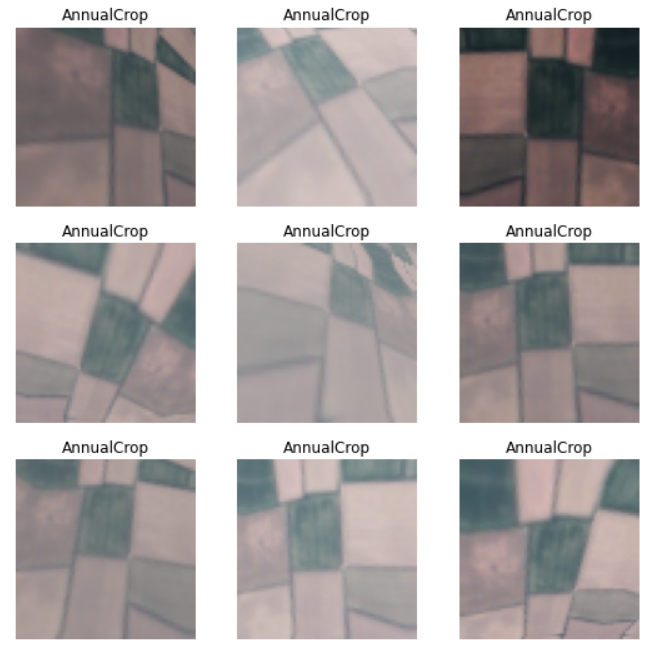
The EuroSAT dataset
The EuroSAT dataset was created at the Deutsches Forschungszentrum für Künstliche Intelligenz (DKFI). The images were extracted from the Sentinel-2A L1C products covering cities in 34 European countries all over a year. The dataset consists of two subsets: RGB and multispectral. Each dataset contains 27000 images divided in 10 classes with 2000 to 3000 images per class. The classes defined to label the images are a subset of those defined in CORINE: Pasture, HerbaceousVegetation, Industrial, AnnualCrop, Residential, PermanentCrop, Highway, SeaLake, Forest, River. The RGB dataset contains images covering the three bands in the visible region of the spectrum (RGB colors). The multispectral dataset contains images covering all the 13 specral bands available from the MSI sensor of the Sentinel-2 satellites. The size of each patch image is 64x64 pixels with 10 m resolution. In this notebook I use only the RGB dataset.
Finetuning a pretrained ResNet architecture
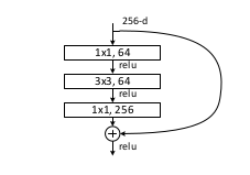
A Convolutional Neural Network that can learn how to distinguish different types of land covers, where geometries and reflectance properties can be mixed in many different ways, requires an architecture with many layers to achieve a good accuracy. Such architectures are expensive to train from scratch in terms of amount of labeled data needed for training, and also in terms of time and computing resources. It is nowadays normal practice in computer vision to reuse a model that has been pretrained on a different but large set of examples, such as ImageNet, and finetune the pretrained model with data that is specific to the task at hand, in our case LULC classification. Finetuning is a transfer learning technique in which the parameters of a pretrained neural network architecture are updated using the new data. I will use the ResNet50 architecture, pretrained on the ImageNet dataset, as suggested in the EuroSAT paper. I will use the fastai deep learning library to implement all the functions required in this notebook. Fastai is a high level library that leverages the underlying PyTorch machine learning framework.
Prepare the development environment
I use Google Colab for development and to test the code using the GPUs that are provided free of charge. The machines available in Google Colab come with an old version of the fastai library that does not support the functions and classes that I will be using and must be updated. I use fastai version 2.5.1 but any other later version should also work fine.
Download the EuroSAT RGB dataset
I download the EuroSAT RGB images from the DKFI website. The images are compressed in a zip file and divided in 10 folders named after the classes defined for the classification task.
Define the DataLoaders, the test and validation set, and the transformations to be applied
The fastai library provides classes and functions to specify the type of example data (images, text files, tabular data), which transformations must be applied on them (e.g. resizing, cropping), how to find the images in the file system, how to extract their labels (classes), and how to split the EuroSAT dataset in a training set and a validation set. We can also artificially increase the number of images using the data augmentation technique. Fastai provides a convenience function that creates more images from the original EuroSAT dataset by applying different transformations such as flipping, rotation, brightness modification and others. I use the fastai default splitting value, 80% for training and 20% for validation. I do not apply any resizing since all the images in EuroSAT used to finetune the pretrained model have the same shape (64x64 pixels). The main step is to transform all the JPG images in PyTorch tensors, i.e. multidimensional float arrays that can be sent in batches to a GPU for computations. The fastai DataBlock class creates batches of images as 4 dimensional tensors for both the training and the validation steps. A batch is a tensor whose dimensions are B x C x H x W where B stands for batch size, C for channels (e.g. the 3 RGB channels), H for height, and W for width. The default batch size for a DataBlock is 64.
blocks = DataBlock(blocks = (ImageBlock, CategoryBlock),
                 get_items=get_image_files, # finds the images in the path
                 splitter=RandomSplitter(seed=42),  # default random split 80% training, 20% validation
                 get_y=using_attr(RegexLabeller(r'(.+)_\d+.jpg$'), 'name'), # extracts the label category from the image's folder name
                 batch_tfms=aug_transforms(mult=2)) # data augmentation (mult multiplies the default transformation values)

dls = blocks.dataloaders(path)
Data augmentation
Additional images have been already created in the previous step from the original ones by using the data augmentation technique implemented by the fastai aug_transforms() convenience function. Here I show the images that are created from one example.
Setup the ResNet50 ConvNet pretrained architecture
Now we select the pretrained architecture to be fine-tuned using the EuroSAT dataset and the metric we want to use to check whether our model achieves our expectations. In this case we use the accuracy as a metric, that can be simply computed from the error rate (accuracy = 1 - error_rate). We use the ResNet50 architecture pretrained with the ImageNet dataset as in the EuroSAT paper. The ResNet50 CNN architecture contains a sequence of blocks. Each block contains from 1 to 3 convolutional layers for a total of 50 convolutional layers.
Each block contains a shortcut connection from the input to the output so that it learns the difference between them, that is the residual. This architectural choice allows to avoid the degradation problem that affects other architectures with many convolutional layers. As said before, a deep architecture is required to learn many complex features from data. Another advantage of the ResNet50 architecture is that the number of parameters don’t depend on the size of the images. The batch size is always the same (64). The number of channels, also known as features maps, increases till the last convolutional layer while the height and width of each channel is decreased by the max pooling layer at the end of each block. The final layer reduces the tensor to a one dimensional vector of size 10, the number of the classes, that is finally sent to a softmax layer that computes the probabilities of each image to be a member of any of the 10 classes used to classify the EuroSAT images. The fastai convenience function cnn_learner() is used to customize the learning process by setting different hyperparameters such as the optimizer (e.g. Stochastic Gradient Descent), the loss function, the learning rate and many others. A summary of the architecture is shown before starting the finetuning process.
Sequential (Input shape: 64)
============================================================================
Layer (type) Output Shape Param # Trainable
============================================================================
64 x 64 x 32 x 32
Conv2d 9408 False
BatchNorm2d 128 True
ReLU
MaxPool2d
Conv2d 4096 False
BatchNorm2d 128 True
Conv2d 36864 False
BatchNorm2d 128 True
____________________________________________________________________________
64 x 256 x 16 x 16
Conv2d 16384 False
BatchNorm2d 512 True
ReLU
____________________________________________________________________________
64 x 256 x 16 x 16
Conv2d 16384 False
BatchNorm2d 512 True
____________________________________________________________________________
64 x 64 x 16 x 16
Conv2d 16384 False
BatchNorm2d 128 True
Conv2d 36864 False
BatchNorm2d 128 True
____________________________________________________________________________
64 x 256 x 16 x 16
Conv2d 16384 False
BatchNorm2d 512 True
ReLU
____________________________________________________________________________
64 x 128 x 16 x 16
Conv2d 32768 False
BatchNorm2d 256 True
____________________________________________________________________________
64 x 128 x 8 x 8
Conv2d 147456 False
BatchNorm2d 256 True
____________________________________________________________________________
64 x 512 x 8 x 8
Conv2d 65536 False
BatchNorm2d 1024 True
ReLU
____________________________________________________________________________
64 x 512 x 8 x 8
Conv2d 131072 False
BatchNorm2d 1024 True
____________________________________________________________________________
64 x 128 x 8 x 8
Conv2d 65536 False
BatchNorm2d 256 True
Conv2d 147456 False
BatchNorm2d 256 True
____________________________________________________________________________
64 x 512 x 8 x 8
Conv2d 65536 False
BatchNorm2d 1024 True
ReLU
____________________________________________________________________________
64 x 256 x 8 x 8
Conv2d 131072 False
BatchNorm2d 512 True
____________________________________________________________________________
64 x 256 x 4 x 4
Conv2d 589824 False
BatchNorm2d 512 True
____________________________________________________________________________
64 x 1024 x 4 x 4
Conv2d 262144 False
BatchNorm2d 2048 True
ReLU
____________________________________________________________________________
64 x 1024 x 4 x 4
Conv2d 524288 False
BatchNorm2d 2048 True
____________________________________________________________________________
64 x 256 x 4 x 4
Conv2d 262144 False
BatchNorm2d 512 True
Conv2d 589824 False
BatchNorm2d 512 True
____________________________________________________________________________
64 x 1024 x 4 x 4
Conv2d 262144 False
BatchNorm2d 2048 True
ReLU
____________________________________________________________________________
64 x 512 x 4 x 4
Conv2d 524288 False
BatchNorm2d 1024 True
____________________________________________________________________________
64 x 512 x 2 x 2
Conv2d 2359296 False
BatchNorm2d 1024 True
____________________________________________________________________________
64 x 2048 x 2 x 2
Conv2d 1048576 False
BatchNorm2d 4096 True
ReLU
____________________________________________________________________________
64 x 2048 x 2 x 2
Conv2d 2097152 False
BatchNorm2d 4096 True
____________________________________________________________________________
64 x 512 x 2 x 2
Conv2d 1048576 False
BatchNorm2d 1024 True
Conv2d 2359296 False
BatchNorm2d 1024 True
____________________________________________________________________________
64 x 2048 x 2 x 2
Conv2d 1048576 False
BatchNorm2d 4096 True
ReLU
____________________________________________________________________________
64 x 512 x 2 x 2
Conv2d 1048576 False
BatchNorm2d 1024 True
Conv2d 2359296 False
BatchNorm2d 1024 True
____________________________________________________________________________
64 x 2048 x 2 x 2
Conv2d 1048576 False
BatchNorm2d 4096 True
ReLU
AdaptiveAvgPool2d
AdaptiveMaxPool2d
Flatten
BatchNorm1d 8192 True
Dropout
____________________________________________________________________________
64 x 512
Linear 2097152 True
ReLU
BatchNorm1d 1024 True
Dropout
____________________________________________________________________________
64 x 10
Linear 5120 True
____________________________________________________________________________
Total params: 25,619,520
Total trainable params: 2,164,608
Total non-trainable params: 23,454,912
Finetuning
Now the ResNet50 architecture is loaded with the pretrained parameters and the finetuning process can start. I set the number of epochs to a value that achieves a good enough accuracy without wasting too much time and resources in computations. We can try different numbers of epochs to find the right one. Fastai provides a convenience function that can do the work for us. In an epoch a batch of images is used to compute an average value of the loss and to update the model parameters before using the next batch till all the batches have been used and a new epoch can start.
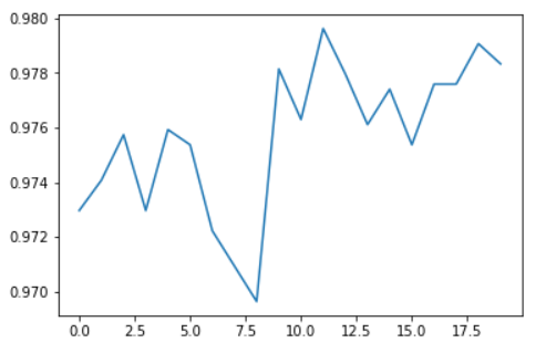
learn.fine_tune(20)
We have achieved an accuracy close to 98%. The exact value can change slightly anytime we finetune the model. If that level of accuracy is enough for our purpose we can stop here otherwise we can run more epochs, try different learning rates or apply more transformations to further increase the number of images. We can plot the accuracy of the finetuned model relative to the number of epochs.
Model evaluation
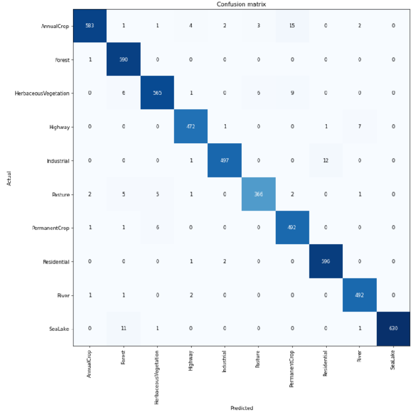
We want to understand what is the accuracy of our model in separating images that belong to different classes. For example, it is known that the spectral response of rivers (turbid water) and roads is pretty similar in the visible part of the spectrum as they absorb most of the solar radiation, and seen from a long distance within a patch of 640 m x 640 m a river and a highway might be confused. So we will not be surprised if some images of rivers and roads may be misclassified, that is, an image of a river may be interpreted as an image of a road and vice versa by our model. Also, the distinction between Pasture, Permanent Crop, Annual Crop or Herbaceous Vegetation may not be so clear using only the three RGB bands so we can expect a certain level of misclassifications among these classes as well. We plot the confusion matrix using the validation data to check for which classes there have been misclassifications.
As we already figured out, most of the misclassifications happen between classes that are related to the vegetation. Also for rivers and highways some misclassifications are reported. Still the great majority of classifications for each class are correct.
A minimalist application
Once we have achieved the accuracy that we wanted, we can use our finetuned model with new images, for example extracted from the Sentinel-2 products available from Sentinel-Hub. I have extracted some patch images of the same size as those used to finetune the model (64x64 pixels). The new images were extracted manually from Sentilel-2 L1C products using the Sentinel-Hub EO-Browser. As an example I use two images from the exact same area from Mesero (Lat. = 45.487971, Lon. = 8.849979), close to Milan, taken two years apart from each other to show how the application can be used to detect changes in land cover and use. The 1st image of the area was taken in July 2019 and shows a land that is mostly covered by crops (‘Permanent Crop’ or ‘Annual Crop’) but also contains a highway at its bottom.
The probabilities computed by our model for the 1st image (Mesero 2019) are:
The model has been able to detect the change of land use and land cover even if the presence of objects of two different classes in the same image, i.e. crop and highway in the 1st image and industrial building and highway in the 2nd image has decreased the confidence of the model.
Conclusion
Thanks to the fastai deep learning library it took less than 1 hour to set up the code, finetune the ResNet50 architecture with the EuroSAT RGB dataset for 20 epochs and also perform some tests using new images extracted from the Sentinel-2 products. We have seen that the performances for an LULC task are already quite good but there is certainly room for improvements. The next step is to use the EuroSAT multispectral dataset with the complete set of the Sentinel-2 MSI 13 spectral bands to see whether it helps in better separating the classes related to crop, pasture and forest where the bands in the Near Infrared (NIR) show a stronger reflectance from vegetation than the visible bands. A Jupyter notebook with the complete Python code is available on my GitHub repository.
The Hough transform is used in digital image processing and computer vision to find geometrical shapes such as lines, circles or ellipses, common in images that contain man-made objects. The Hough transform can be used after an image has been pre-processed by an edge detector to find the edges that reveal the border of objects or regions inside it. In this post I will introduce briefly the theory behind the Hough transform, and then I will present two examples , one with images containing simple geometrical shapes, to better explain the idea, and one with an image containing man-made objects. A Jupyter notebook with the Python code used to implement the functions discussed in the post and to derive the pictures shown here is available on my GitHub repository.
Introduction
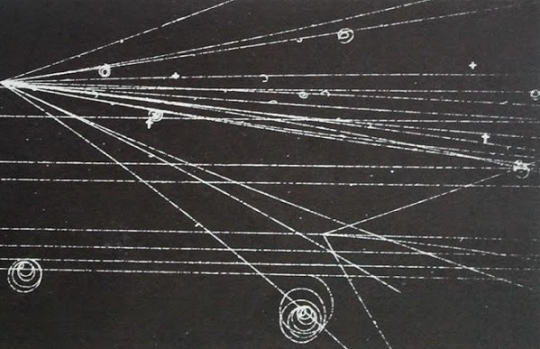
In digital image processing different filters are available that can detect edges on an image, namely regions in which the intensity value of a set of pixels along a certain direction changes steeply. These regions contain pixels that are members of real edges but also pixels that are due to noise or blurring. Often what we want to know, and what we want a computer to detect, is the shape, namely the analytical description of the object that has been revealed by the edge detector, such as the slope and intersect of a line. This further step, after the edge detection, is called edge linking and consists of connecting together the pixels that are real members of an edge of a certain shape, avoiding the pixels that have been included due to noise or blurring. The most common shape that can be found in pictures, especially those containing man-made objects, is a line. The problem can be solved by exhaustively by testing all the pixels in the edge regions. However, the computational complexity of such an approach would be proportional to the square of the number of edge pixels. Another approach was suggested in 1962 by Paul Hough, while trying to automatically determine the trajectories of charged particles crossing a bubble chamber.
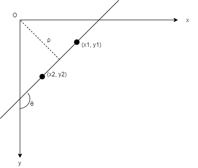
The Hough method was to transform each bubble point $(x_0, y_0)$, represented by a pixel in the image, and the set of all possible lines $y_0 = sx_0 + d$ passing through it, into a line in a parameter space $(s, d)$ whose variable were the slope $s$ and the intercept $d$ with the y axis. If two points in the image belong to the same line, their representations in the parameter space must intersect for a certain value of the slope $s$ and the intercept $d$. We can therefore solve the problem of finding a line that goes through a certain number of pixels in the image by solving the problem of finding the point in the parameter space where the lines that represent each pixels intersect. The more lines intersect in a specific point $(s_0, d_0)$ of the parameter space, the more pixels in the image belong to the same line with slope $s_0$ and intersect $d_0$. The point in the parameter space that lies at the intersection of a high number of lines represents the most “voted” line in the image. Since the linear parametrization is unbounded for vertical or near vertical lines, a different transformation was introduced by Duda and Hart that uses as parameters the orientation angle $\theta$ and the distance $\rho$ from the origin of the coordinates system to represent the set of lines that can pass through a pixel. We can derive the normal form of a line by computing the slope and the intercept in the frame of reference that is commonly used for images where the origin is on the upper left corner, with the y axis pointing downward and the x axis pointing to the right.
From the diagram we can easily derive the expressions of the slope s and the intercept d for the equation of a line $y = sx + d$
so that we can represent the set of lines passing through a pixel at $(x_0, y_0)$ with the expression
\[\rho = -x_0 cos(\theta) + y_0 sin(\theta)\]
With this expression, called normal Hesse form or simply normal form, we can represent the set of lines that pass through a pixel at $(x_0, y_0)$ in the image by a sinusoidal function in the parameter space $(\theta, \rho)$. If two points belong to the same line in the image, their representations as sinusoidal functions in the parameter space must intersect at a certain point $(\theta_0, \rho_0)$. Similarly to what has been said before, the more sinusoidal curves intersect in a point $(\theta_0, \rho_0)$ of the parameter space, the more its corresponding line in the image ranks high enough to be elected as a real line. We can count the number of sinusoidal curves that intersect at each point of the parameter space by dividing this space into a grid of cells whose width and height depends on the angular and spatial resolution of the image. For example, if we can distinguish two lines in the image that are rotated by 1 degree and two lines that are separated by one pixel, we can set the width of each cell in the parameter space $(\theta, \rho)$ as one degree and the height as 1 pixel. In Python we can use a two-dimensional array to store the number of sinusoidal curves that pass through each cell. The 2D array is called accumulator matrix. Once we have processed all the edge pixels, computed the corresponding Hough transform and counted the votes for each cell in the accumulator matrix, we can select the cells that contain the highest number of votes that correspond to straight lines in the image.
In the following section we will see examples of the application of the Hough transform to detect simple geometrical shapes, made up of dotted lines.
Images with geometrical shapes
An image in Python is a 2D array in which the intensity values of each pixel are stored. We start by creating an image with shapes composed of lines to test the performances of the Hough algorithm. The first step is to compute the Hough transform, in normal form, for each pixel that belongs to a geometrical shape. The second step is to initialize the accumulator matrix $A$ and, for each pixel that belongs to a shape, mark each cell $A[i_{\rho}, j_{\theta}]$ in the accumulator that is passed by its Hough transform, represented by a sinusoidal curve. In other words, we store in the accumulator the trace of the Hough transform of every edge pixel in the image. The Hough transform returns the quantized values $j_{\theta}$ and $i_{\rho}$ for $\theta$ and $\rho$. We choose the quantization for the angle $\theta$ based on the accuracy of the orientation of a line in the image. We assume the angle $\theta$ lies in the interval $0 \leq \theta \lt 180$ so that the relation between $\theta$ and $\rho$ is one-to-one. If the resolution of our image is good enough that we can distinguish lines whose difference in slope is at least one degree, we can set the increment to 1 degree, or $\frac{\pi}{180}$ radians.
In the same way, we can choose the quantization for the distance $\rho$ of a pixel from the origin. Given an image whose 2D array shape is (M,N), i.e. M rows and N columns, the distance between any two pixels in the image cannot be bigger than the length of the diagonal of the image, therefore $0 \lt \rho \lt \sqrt{M^2 + N^2}$. If the spatial resolution of our image is one pixel, we can set the increment for the distance to 1 pixel as well.
With this quantization we can represent any pixel in an image and the set of lines that pass through it, represented by the parameters $\theta$ and $\rho$ in the parameters space, with the two integer values $j_{\theta}$ and $i_{\rho}$ that can range between 0 and 180 degree and 0 and the length of the diagonal of the image, respectively. The two integer values are used as indexes of the cell $A[i_{\rho}, j_{\theta}]$ that contains the number of votes for the line in the image whose angle with the y axis is $\theta$ and whose distance from the origin is $\rho$.
The Hough curves
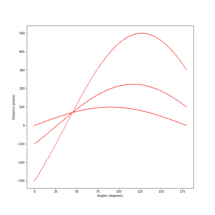
As an example, we plot the Hough sinusoidal curves of three aligned pixels, to see that they intersect in one point $(\theta_0, \rho_0)$ of the parameter space that corresponds to the angle $\theta_0$ between the line that passes through them and the y axis, and to the distance $\rho_0$ of the line from the origin.
We can see from the plot that the three sinusoidal curves that represent the three pixels in the parameter space cross each other at 45 degrees and at a distance of approximately 70 pixels. We will see how to use the accumulator matrix to derive both values with the best accuracy possible. The picture can be seen as a snapshot of the accumulator matrix, after the Hough transforms of the three pixels have been determined and stored.
The accumulator matrix
As said before, in Python we can use a 2D array to store the traces of the curves computed for each edge pixels using the Hough transform. We can see that the value of the distance parameter $\rho$ can be negative for certain values of the pixel coordinates and of the angle $\theta$. Since NumPy cannot use negative values for indexes we get the absolute value of the distance. In this way we will be able to store the votes for any point in the parameters space.
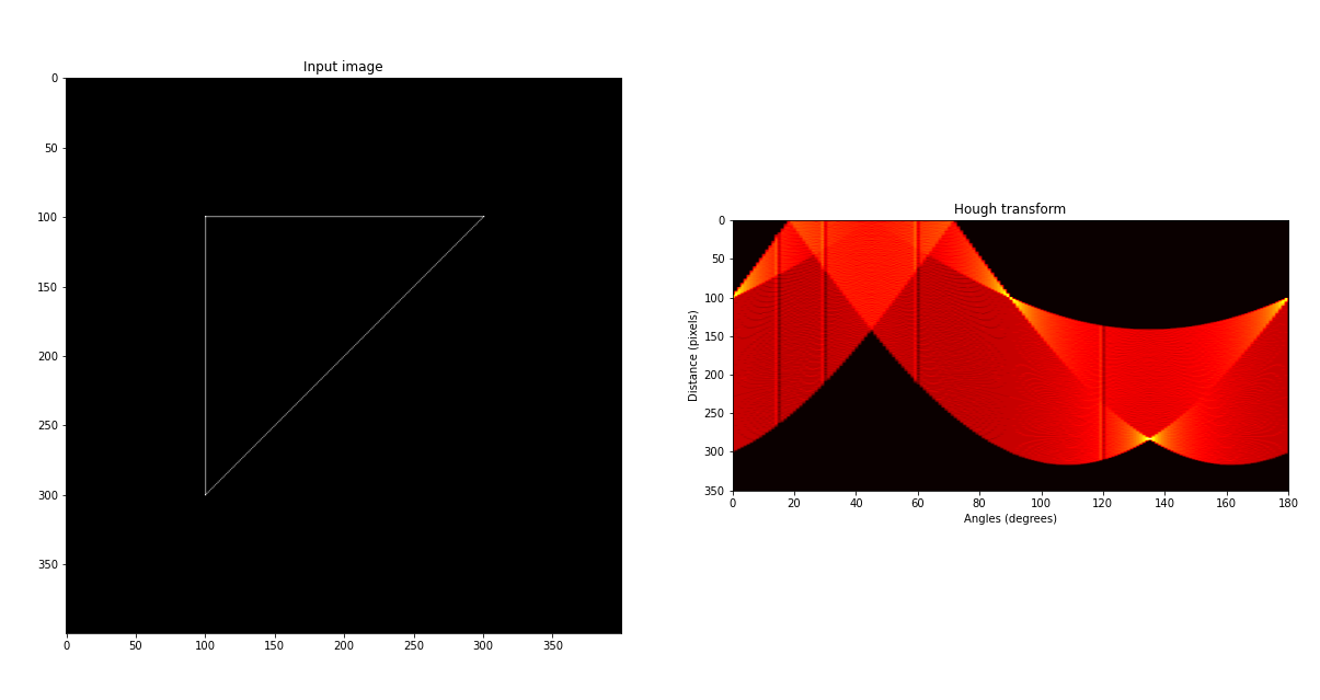
We create an image with a triangular shape and then we compute the Hough transform of each pixel that belongs to any of the three lines that form the triangle. We store the number of curves that pass through each accumulator’s cell $A[i_{\rho}, j_{\theta}]$ and, after all the edge pixels are processed, we plot the image and the corresponding accumulator matrix. We notice four points in the Hough transform diagram with the highest values, also called peaks: the point at 135 degrees, that has the highest number of votes, one at 90 degree, that represents the horizontal line in the image, and two other points at 0 and 180 degree that represent the same vertical line in the image. We can extract the peaks from the accumulator matrix by setting a minimum vote threshold and taking only the cells whose value lies above it.
After we have got the angle $\theta$ and distance $\rho$ of the peaks in the accumulator matrix, corresponding to the most voted lines in our image, we can compute the respective slopes and intercepts.
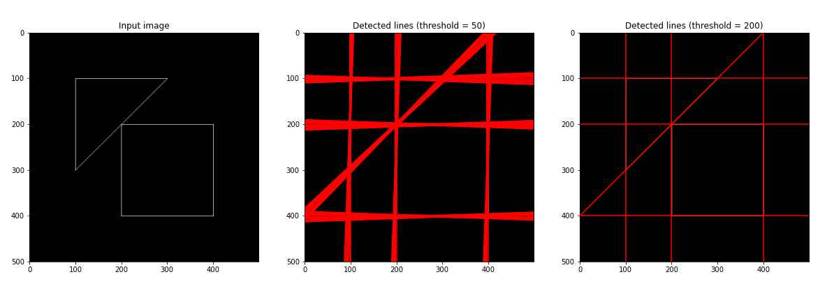
We show another example with an image that contains a little more complex figure with two geometrical shapes, the triangle we have already used and a square box. We create the image and compute the accumulator matrix. We plot the image and the detected lines setting the minimum threshold for the cells in the accumulator matrix to 50 votes first and then to 200.
Images with man-made objects
Now that we have tested our implementation of the Hough transform with images containing geometrical shapes made up of dotted lines, we are ready to move on to the next step, namely, applying the algorithm to find lines in pictures containing man-made objects. When we use pictures of real objects, before looking for lines or other geometrical shapes, we have to detect the edges that reveal the border of objects or regions in the image. This step was not necessary in the previous examples because the edges of the geometrical shapes were drawn precisely using the equation of a line. Borders separating man-made or natural objects can be found using a thresholding function or an edge detector. Once edges have been detected, the next step is to link their pixels to find out lines for which we can determine the slope and the intercept. We perform the linking step using the Hough transform. We can build a pipeline of functions to find lines in pictures. We can add one more step to our pipeline to take into account the quantization error of the accumulator matrix for which the Hough lines may not intersect exactly in one single cell but more likely in a cluster of neighboring cells. We add a thresholding step after the edge detector to separate precisely the edges from the background. The complete steps that we will perform in the next example are the followings
Apply the gradient-based edge detector to an image to get its edge map.
Apply a threshold to the edge map to obtain a binary representation.
Apply the Hough transform to the foreground pixels of the binary edge map to build the accumulator matrix.
Suppress the nonmaximal cells from the accumulator matrix to reduce the quantization error
Set the minimum votes threshold to select the peaks in the accumulator matrix that correspond to straight lines in the image.
Compute the slopes and intercepts of the lines in the image corresponding to the peaks.
Plot the lines on the image.
The quantization error can be addressed by suppressing from the accumulator matrix the nonmaximal cells whose value is lower than any of its neighboring cells. A function is defined in the Jupyter notebook to implement the suppression of the nonmaximal cells.
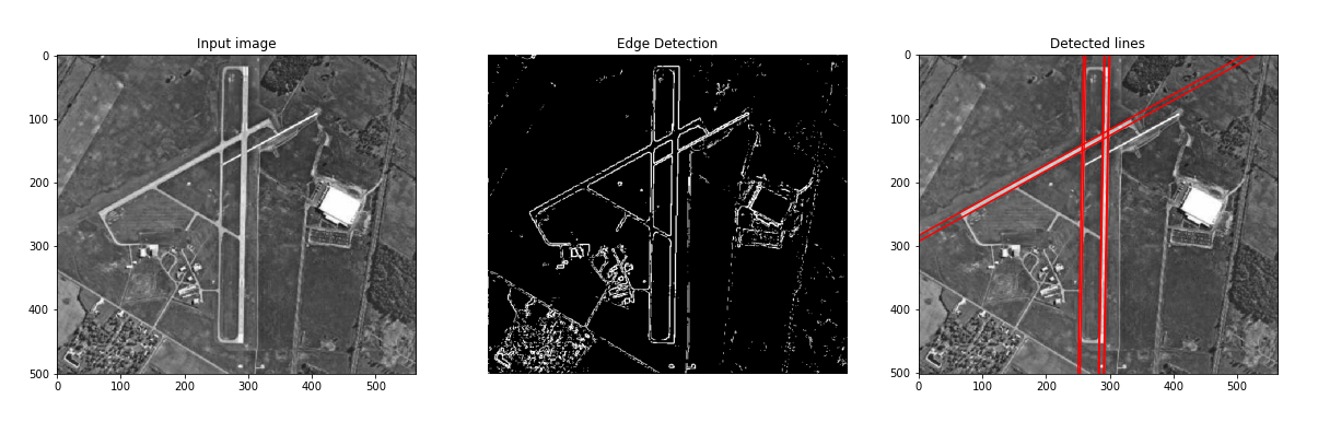
In the next example we use an image of an airport that contains two runways, among other structures. We compute the edge map of the image by applying a gradient filter, and then we create a binary version of the edge map by applying a thresholding function that enhances the separation between the edges and the background. From the binary edge map we can compute the accumulator matrix. We suppress the nonmaximal cells in the accumulator matrix, within a default distance of one pixel from each cell and finally, we select the peaks in the parameter space whose number of votes are above a threshold. The slopes and intercepts corresponding to the peaks are used to plot the detected lines superimposed on the original image.
We can see from the last picture that the Hough transform is able to determine the main lines, with their slopes and intercepts, that correspond to the borders of the runways of the airport. We can also notice that other lines, visible in the binary image, have not been included in the set that resulted from our choice of the vote threshold and neighboring distance. This is mainly due to the fact that those lines are shorter or contain less edge pixels than the two runways. This bias towards longer lines can be addressed, for example by dividing the image in smaller boxes and then applying the Hough transform to each of them, or by finding the pixels that delimit the lines in the binary image and then looking for the corresponding lines in the accumulator matrix.
Conclusion
The Hough transform can be used to extract lines from images with a complexity cost that is linear with respect to the number of edge pixels. We have shown the basic steps that are required to implement the Hough transform for which some manual settings are required, such as the quantization of the parameter space, the votes threshold and the neighboring distance for the accumulator matrix.